When It Rains It Pours
#23: Covariance and Convexity in Financial Models.
This week, we will explore the mechanics and pitfalls of financial modeling through the lens of a private equity leveraged buyout (LBO). Why do models often fail to predict common outcomes?
The Paper LBO
Close your eyes and picture the scene.
It’s 9:30AM on a Thursday morning. You, a 23 year-old sleep-deprived investment banking analyst, told your desk you would be out for the morning getting a cavity filled - an unoriginal excuse - but instead, you are sitting in a glass-paneled office overlooking Midtown Manhattan. The interviewer sitting across from you, a mid-level private equity professional, asks you to take out a blank sheet of paper.
You know what’s coming, you’ve practiced for it. She begins:
Consider a company with the following characteristics:
$50 million in revenue next year growing at 10% per year
20% EBITDA margins
$4 million of capital expenditures (capex) and depreciation & amortization (D&A) per year, growing in line with revenue
No working capital
40% tax rate
Now, assume you can buy the company at 10x forward EBITDA, using 5x leverage at a 5% interest rate, and sell the company in 5 years at the same multiple. What is your return?
After frantically scribbling down the prompt, you get to work.
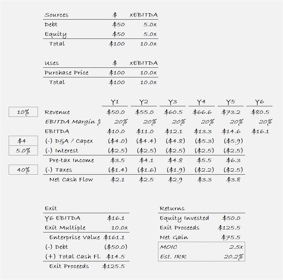
First, build a sources and uses table, to determine the purchase price and how the transaction will be funded1. Second, project each of the line items from revenue down to net cash flow2. Then, calculate the net proceeds you will receive in year 5 based on the exit multiple and net debt outstanding3. Finally, compare your net proceeds to your initial investment to calculate the return4.
By the end of the exercise, your paper looks like this:
You can now answer the interviewer’s question. You invest $50 million of equity to buy the company and receive $125.5 million at exit - a 2.5x multiple of invested capital (MOIC). A 2.5x return on capital over five years is a 20% internal rate of return (IRR) - a relationship that you’ve memorized in advance.
This exercise, known as a “paper LBO”, is ubiquitous in private equity interviews because it captures the business model in a nutshell. To answer the question, you must be able to mechanically lay out an LBO model, calculate net cash flows, complete some mental math, and have an understanding of investment returns.
Yet, like any model, even a paper LBO is only as good as its assumptions.
Components of Return
A typical follow up question to a paper LBO is to disaggregate the drivers of the $75.5 million gain on the investment. The textbook response says there are three elements of return:
Growth: In our example, EBITDA grew from $10 million to $16.1 million, or $6.1 million over the hold period. When applying the 10x EBITDA multiple to this growth, we see that growth accounts for $61.1 million of the gain on investment.
Cash Flow: The company generated $14.5 million of cash flow during the hold period.
Exit Multiple: Because we assume that we enter and exit the investment at a 10x multiple, there is no gain or loss associated with the exit multiple.
Based on this breakdown, we see that the growth assumption drives nearly all of the investment return, while actual cash generated during the hold period is only a minor contributor. Our assumption of exit/entry parity has no bearing on return.
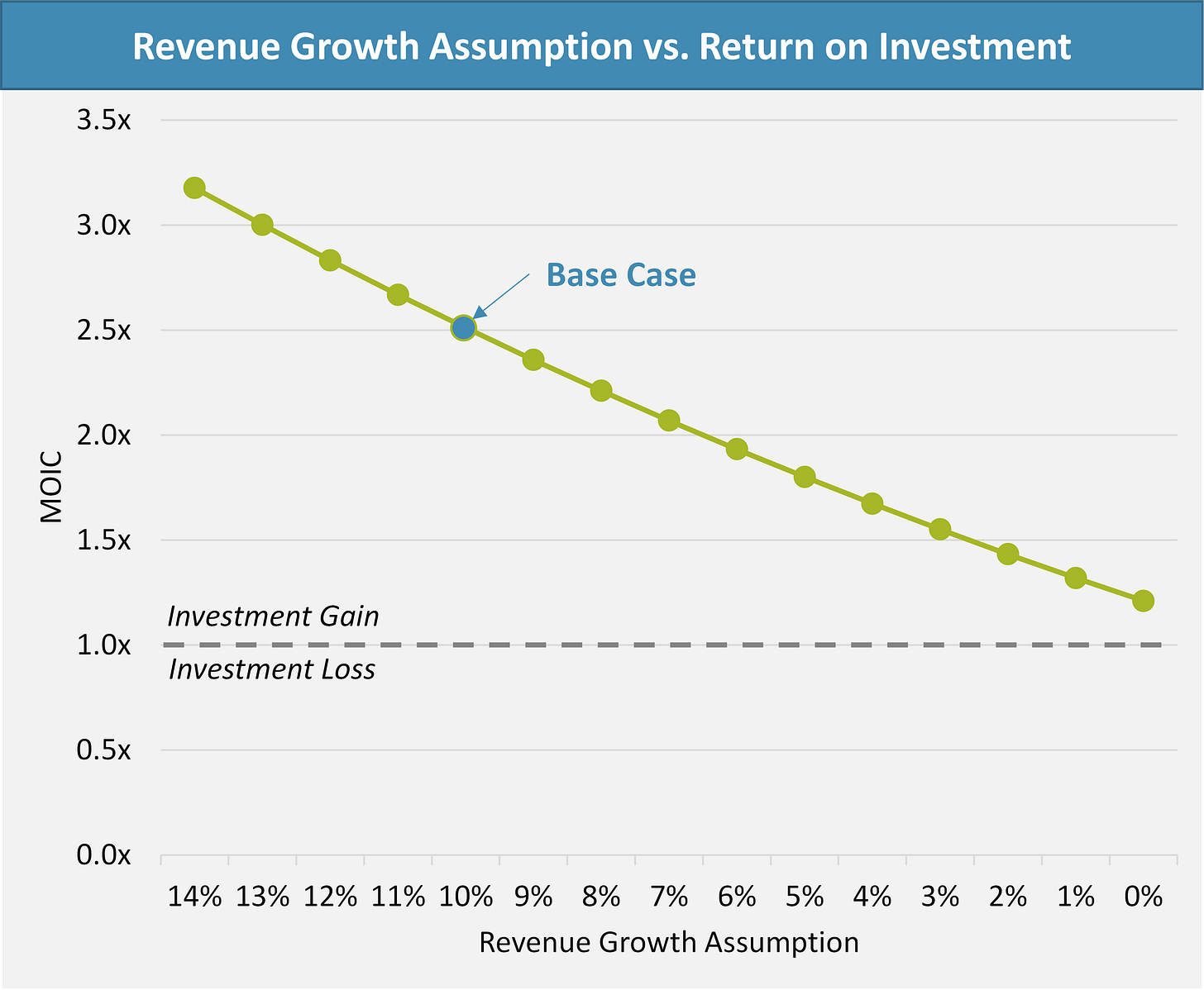
Knowing that the investment hinges heavily on the growth assumptions, it makes sense to sensitize this variable to see how deviations from expectations impact returns. When holding all other variables constant and changing the assumed revenue growth, we see that revenue growth has a near linear impact on investment returns.
While this analysis shows that investment returns are highly dependent on revenue growth, it also suggests a surprisingly resilient investment profile. If you were to totally whiff on your assumptions, and the company does not grow at all, you would still have a marginally profitable investment (driven by cash flow during the period).
In reality, this is almost certainly not the case. If you underwrite a private equity investment to a 20% return assuming 10% compounded growth, and the company does not grow at all, you will likely lose a lot of money.
Covariance and Convexity
The simple breakdown of LBO returns into growth, cashflow, and exit multiple is a useful mathematic bridge but creates a false sense of independence between the variables. In reality, all of the variables are correlated and cannot be separated in such a simplistic sense. For one, revenue growth rate will impact the cash flow generated during the hold period. More important is the impact on the exit multiple.
The universal convention in LBO modeling is to assume parity in exit and entry multiples. This is often considered “conservative” in the sense that you don’t assume multiple expansion in your base case. It is also true that if a company was to continue growing at your initial growth assumptions, then a subsequent buyer with the same cost of capital should pay the same multiple for the business.
But, while multiple parity is a justifiable base case assumption, it cannot be assumed to be static. Rather, the exit multiple must flex along with the actual performance of the business. If the business only grows at 5% instead of 10%, this will reduce the EBITDA growth and cash flow during the hold period but also cause multiple contraction at exit. Alternatively, if the business outperforms, a subsequent buyer should be willing to pay a higher multiple.
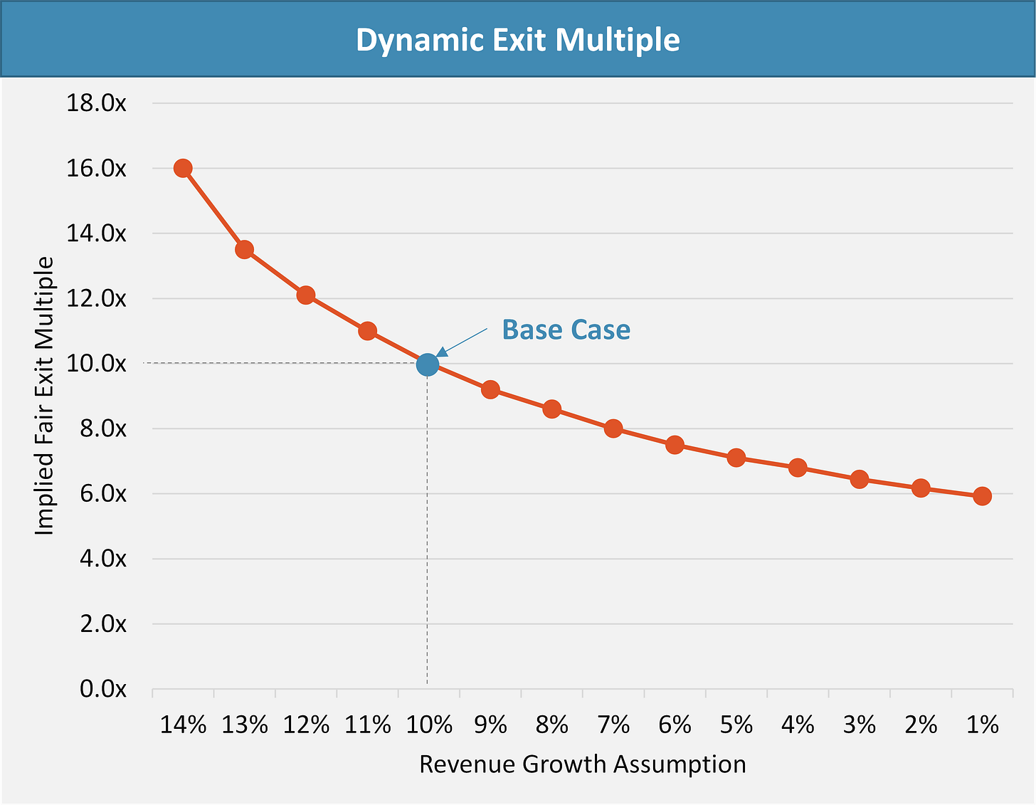
If we assume a subsequent buyer has the same cost of capital as the initial buyer (i.e. requires the same 20% return), we can create a dynamic exit multiple assumption that incorporates the actual growth of the business during the hold period5.
There is a non-linear relationship between the company’s growth rate and the multiple the next buyer could pay to achieve a 20% return, assuming the buyer extrapolated the growth rate going forward.
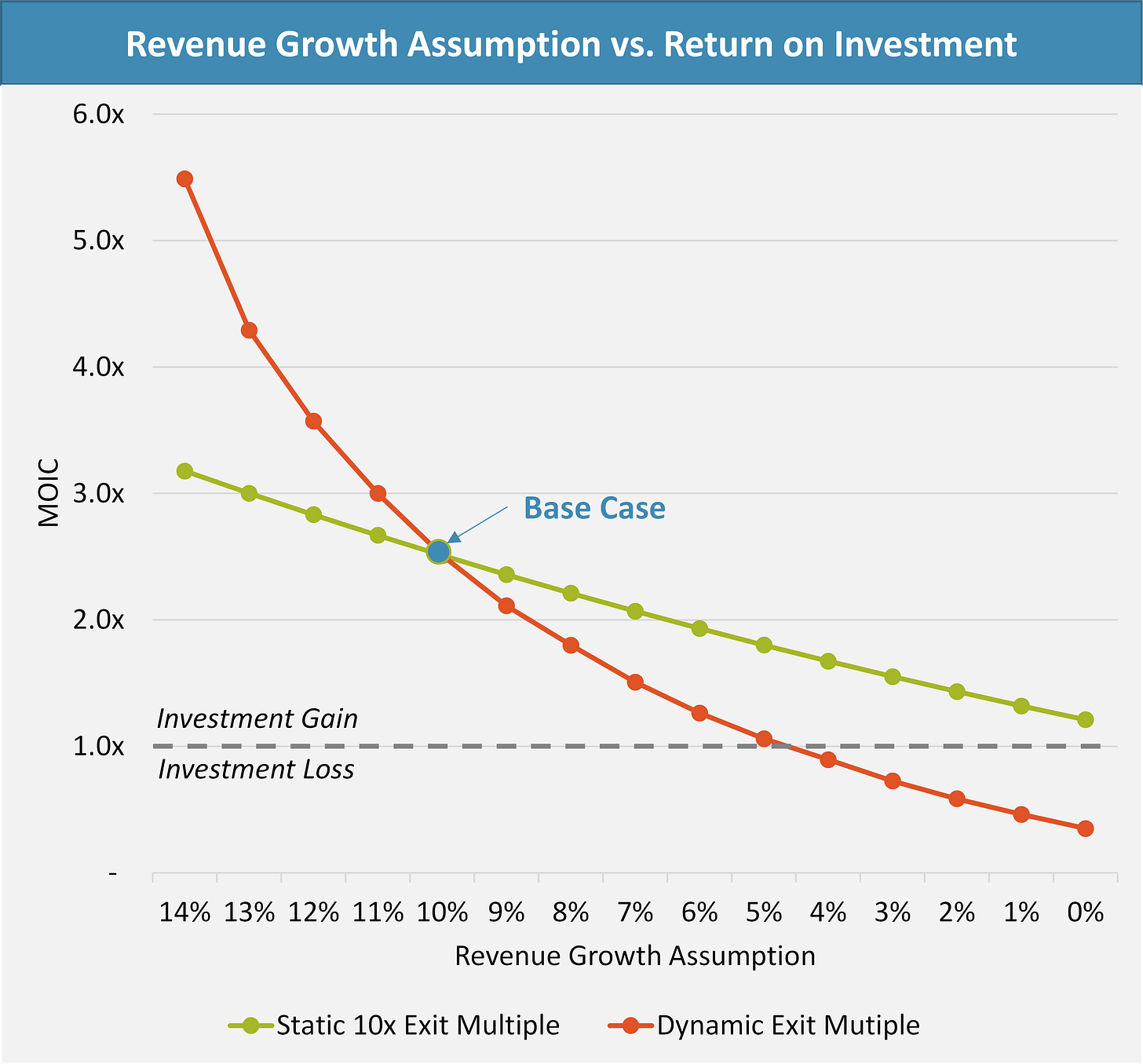
Now, we can re-run our previous revenue growth sensitivity to include both its impact to the cash flows during the hold period as well as its implications for exit valuation.
By incorporating the covariance of revenue growth and exit multiples, the dynamic sensitivity shows a convex line with far more upside and downside. The two curves intersect on the base case assumption. If the company outperforms on growth, multiple expansion juices returns. If the company underperforms though, multiple compression leads to much lower returns. When it rains, it pours.
Unlike the static approach, which shows a small positive return in the zero-growth case, the dynamic exit multiple shows that company must achieve at least a 5% growth rate in order for the investment to be profitable. If the company has no growth, the MOIC falls to just 0.35x, or a loss of 65% of principal.
These two conventions paint starkly different risk and reward profiles. The static multiple implies a range-bound return profile with little risk of principal loss, while the dynamic multiple shows the investment’s true colors - a highly levered investment contingent on strong future growth.
Conclusion
Investment decision are analyzed and iterated ad nauseum. A deal team will present pages of detailed model outputs, backed by endless assumptions, inputs, and calculations from overflowing excel files. Yet, the end result is always the same - the Base Case looks good, the Upside Case is a bit better, and the Worst Case Scenario is not all that bad.
Never will you see a 10-bagger or a complete donut in a memo, yet both these outcomes happen regularly. One key failure is the tendency to think about assumptions as independent (and often counterbalancing), when in reality they row in the same direction, compounding moves in good and bad directions. Better models incorporate covariance and convexity and the volatility each brings.
As always, thank you for reading. If you enjoy The Last Bear Standing, tell a friend! And please, let me know your thoughts in the comments - I respond to all of them.
-TLBS
You buy the company for $100 million (10 x $10 million in EBITDA), funded with $50 million in debt (5 x $10 million in EBITDA) and the remaining $50 million with equity.
Multiply revenue by 20% margins to get EBITDA, then subtract capex, interest, and taxes to get cash flow. Because D&A is equal to capex in this example, the calculations of pre-tax income and cash flow can be simplified. If the two figures were different, you would need to subtract D&A to calculate pre-tax income, then add back D&A and subtract capex in the cash flow.
Multiply Year 6 EBITDA of $16.1 by 10 to calculate the gross exit proceeds of $161.1 million. Then subtract your debt ($50 million), and add the cumulative cash flow from the investment period ($14.5 million) to calculate net proceeds.
Divide the $125.2 million exit proceeds by the $50 million investment to determine a multiple of invested capital of 2.5x. Memorizing a cheat sheet of MOIC vs. IRR conversions.
Assumes the subsequent buyer also purchases with 5.0x leverage at a 5% interest rate.


Thank you Bear! This is a great lesson!
Thanks for throwing that one in. Appreciate a glimpse into the VC side of things!